pygmt.Figure.histogram

Figure.histogram(data, bar_width=None, bar_offset=None, cmap=False, pen=None, fill=None, horizontal=False, center=False, out_range=None, stairs=False, cumulative=False, projection=None, region=None, frame=False, verbose=False, panel=False, incols=None, perspective=False, transparency=None, **kwargs)

Calculate and plot histograms.

Full GMT docs at https://docs.generic-mapping-tools.org/6.7/histogram.html.

Aliases:

D = annotate
N = distribution
T = series
Z = histtype
b = binary
d = nodata
e = find
h = header
l = label

w = wrap
A = horizontal
B = frame
C = cmap
E = bar_width, +o: bar_offset
G = fill
J = projection
L = out_range
Q = cumulative

R = region
S = stairs
V = verbose
W = pen
c = panel
i = incols
p = perspective
t = transparency

Parameters:

data (str | PathLike | dict | ndarray | DataFrame | Dataset | GeoDataFrame) – Pass in either a file name to an ASCII data table, a Python list, a 2-D numpy.ndarray, a pandas.DataFrame, an xarray.Dataset made up of 1-D xarray.DataArray data variables, or a geopandas.GeoDataFrame containing the tabular data.
cmap (str | bool, default: False) – File name of a CPT file or a series of comma-separated colors (e.g., color1,color2,color3) to build a linear continuous CPT from those colors automatically.
pen (str | None, default: None) – Draw bar outline (or stair-case curve) using the specified pen thickness [Default is no outline].
fill (str | Pattern | None, default: None) – Set color or pattern for filling bars [Default is no fill].
annotate (bool or str) – [+b][+ffont][+ooff][+r]. Annotate each bar with the count it represents. Append any of the following modifiers: Use +b to place the labels beneath the bars instead of above; use +f to change to another font than the default annotation font; use +o to change the offset between bar and label [Default is "6p"]; use +r to rotate the labels from horizontal to vertical.
bar_width (float | str | None, default: None) – Use an alternative histogram bar width than the default set via series. Give either an alternative width in data units, or the user may append a dimension unit for a fixed dimension instead.
bar_offset (float | str | None, default: None) – Shift all bars along the axis by a constant value. It may be given in data units of plot dimension units by appending the relevant unit. Requires bar_width.
center (bool, default: False) – Center bin on each value specified via series [Default uses the values to define the left edge of each bin].
distribution (bool, float, or str) –
[mode][+ppen]. Draw the equivalent normal distribution; append desired pen [Default is "0.25p,black,solid"]. The mode selects which central location and scale to use:
- 0 = mean and standard deviation [Default];
- 1 = median and L1 scale (1.4826 * median absolute deviation; MAD);
- 2 = LMS (least median of squares) mode and scale.
out_range (Literal['first', 'last', 'both'] | None, default: None) –
Handle values that fall outside the range set by series. By default, these values are ignored. Valid values are:
- "first": only include values below first bin into the first bin
- "last": only include values above the last bin into that last bin
- "both": include values into the first or last bins
cumulative (bool | Literal['reverse'], default: False) – Pass True to draw a cumulative histogram, or set it to "reverse" to draw a reverse cumulative histogram instead.
stairs (bool, default: False) – Draw a stairs-step diagram which does not include the internal bars of the default histogram.
horizontal (bool, default: False) – Plot the histogram horizontally from x = 0 [Default is vertically from y = 0]. The plot dimensions remain the same, but the two axes are flipped, i.e., the x-axis is plotted vertically and the y-axis is plotted horizontally.
series (int, str, or list) – [min/max/]inc[+n]. Set the interval for the width of each bar in the histogram.
histtype (int or str) –
[type][+w]. Choose between 6 types of histograms:
- 0 = counts [Default]
- 1 = frequency_percent
- 2 = log (1.0 + count)
- 3 = log (1.0 + frequency_percent)
- 4 = log10 (1.0 + count)
- 5 = log10 (1.0 + frequency_percent).
To use weights provided as a second data column instead of pure counts, append +w.
projection (str | None, default: None) – projcode[projparams/]width|scale. Select map projection.
region (Sequence[float | str] | str | None, default: None) – [xmin, xmax, ymin, ymax] or xmin/xmax/ymin/ymax[+r][+uunit]. Specify the region of interest.
frame (Frame | Axis | Literal['none'] | str | Sequence[str] | bool, default: False) – Set frame and axes attributes for the plot. It can be a bool, "none", a pygmt.params.Frame or pygmt.params.Axis object. Raw GMT strings or sequences of strings are also supported for backward compatibility. If frame=True, the frame will be drawn with the default attributes. If frame="none", no frame will be drawn. Use a pygmt.params.Frame or pygmt.params.Axis object for more control over the attributes of the frame and axes. A tutorial is available at frame and axes attributes. Full documentation is at https://docs.generic-mapping-tools.org/6.7/gmt.html#b-full.
verbose (Literal['quiet', 'error', 'warning', 'timing', 'info', 'compat', 'debug'] | bool, default: False) – Select verbosity level [Full usage].
binary (bool or str) –
i|o[ncols][type][w][+l|b]. Select native binary input (using binary="i") or output (using binary="o"), where ncols is the number of data columns of type, which must be one of:
- c: int8_t (1-byte signed char)
- u: uint8_t (1-byte unsigned char)
- h: int16_t (2-byte signed int)
- H: uint16_t (2-byte unsigned int)
- i: int32_t (4-byte signed int)
- I: uint32_t (4-byte unsigned int)
- l: int64_t (8-byte signed int)
- L: uint64_t (8-byte unsigned int)
- f: 4-byte single-precision float
- d: 8-byte double-precision float
- x: use to skip ncols anywhere in the record
For records with mixed types, append additional comma-separated combinations of ncols type (no space). The following modifiers are supported:
- w after any item to force byte-swapping.
- +l|b to indicate that the entire data file should be read as little- or big-endian, respectively.
Full documentation is at https://docs.generic-mapping-tools.org/6.7/gmt.html#bi-full.
panel (int | Sequence[int] | bool, default: False) –
Select a specific subplot panel. Only allowed when used in Figure.subplot mode.
- True to advance to the next panel in the selected order.
- index to specify the index of the desired panel.
- (row, col) to specify the row and column of the desired panel.
The panel order is determined by the Figure.subplot method. row, col and index all start at 0.
nodata (str) – i|onodata. Substitute specific values with NaN (for tabular data). For example, nodata="-9999" will replace all values equal to -9999 with NaN during input and all NaN values with -9999 during output. Prepend i to the nodata value for input columns only. Prepend o to the nodata value for output columns only.
find (str) – [~]“pattern” | [~]/regexp/[i]. Only pass records that match the given pattern or regular expressions [Default processes all records]. Prepend ~ to the pattern or regexp to instead only pass data expressions that do not match the pattern. Append i for case insensitive matching. This does not apply to headers or segment headers.
header (str) –
[i|o][n][+c][+d][+msegheader][+rremark][+ttitle]. Specify that input and/or output file(s) have n header records [Default is 0]. Prepend i if only the primary input should have header records. Prepend o to control the writing of header records, with the following modifiers supported:
- +d to remove existing header records.
- +c to add a header comment with column names to the output [Default is no column names].
- +m to add a segment header segheader to the output after the header block [Default is no segment header].
- +r to add a remark comment to the output [Default is no comment]. The remark string may contain \n to indicate line-breaks.
- +t to add a title comment to the output [Default is no title]. The title string may contain \n to indicate line-breaks.
Blank lines and lines starting with # are always skipped.
incols (int | str | Sequence[int | str] | None, default: None) –
Specify data columns for primary input in arbitrary order. Columns can be repeated and columns not listed will be skipped [Default reads all columns in order, starting with the first (i.e., column 0)].
- For a sequence: specify individual columns in input order (e.g., incols=(1, 0) for the 2nd column followed by the 1st column).
- For a string: specify individual columns or column ranges in the format start[:inc]:stop, where inc defaults to 1 if not specified, with columns and/or column ranges separated by commas (e.g., incols="0:2,4+l" to input the first three columns followed by the log10-transformed 5th column). To read from a given column until the end of the record, leave off stop when specifying the column range. To read trailing text, add the column t. Append the word number to t to ingest only a single word from the trailing text. Instead of specifying columns, use incols="n" to simply read numerical input and skip trailing text. Optionally, append one of the following modifiers to any column or column range to transform the input columns:
  - +l to take the log10 of the input values.
  - +d to divide the input values by the factor divisor [Default is 1].
  - +s to multiple the input values by the factor scale [Default is 1].
  - +o to add the given offset to the input values [Default is 0].
label (str) – Add a legend entry for the symbol or line being plotted. Full documentation is at https://docs.generic-mapping-tools.org/6.7/gmt.html#l-full.
perspective (float | Sequence[float] | str | bool, default: False) –
Select perspective view and set the azimuth and elevation of the viewpoint.

Accepts a single value or a sequence of two or three values: azimuth, (azimuth, elevation), or (azimuth, elevation, zlevel).
- azimuth: Azimuth angle of the viewpoint in degrees [Default is 180, i.e., looking from south to north].
- elevation: Elevation angle of the viewpoint above the horizon [Default is 90, i.e., looking straight down at nadir].
- zlevel: Z-level at which 2-D elements (e.g., the plot frame) are drawn. Only applied when used together with zsize or zscale. [Default is at the bottom of the z-axis].
Alternatively, set perspective=True to reuse the perspective setting from the previous plotting method, or pass a string following the full GMT syntax for finer control (e.g., adding +w or +v modifiers to select an axis location other than the plot origin). See https://docs.generic-mapping-tools.org/6.7/gmt.html#perspective-full for details.
transparency (float | None, default: None) – Set transparency level, in [0-100] percent range [Default is 0, i.e., opaque]. Only visible when PDF or raster format output is selected. Only the PNG format selection adds a transparency layer in the image (for further processing).
wrap (str) –
y|a|w|d|h|m|s|cperiod[/phase][+ccol]. Convert the input x-coordinate to a cyclical coordinate, or a different column if selected via +ccol. The following cyclical coordinate transformations are supported:
- y: yearly cycle (normalized)
- a: annual cycle (monthly)
- w: weekly cycle (day)
- d: daily cycle (hour)
- h: hourly cycle (minute)
- m: minute cycle (second)
- s: second cycle (second)
- c: custom cycle (normalized)
Full documentation is at https://docs.generic-mapping-tools.org/6.7/gmt.html#w-full.

Examples

>>> import numpy as np
>>> import pygmt
>>> # Generate random data from a normal distribution
>>> rng = np.random.default_rng(seed=100)
>>> data = rng.normal(loc=100, scale=25, size=1024)
>>> fig = pygmt.Figure()
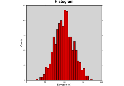
>>> fig.histogram(data=data, frame=True, series=5, fill="red3", pen="1p")
>>> fig.show()